Libraries

First, let’s load some of the libraries that we’ll need.

library(rgl)
library(rayshader)

## Warning: package 'rayshader' was built under R version 3.6.2

library(raster)

## Warning: package 'raster' was built under R version 3.6.2

library(sp)
library(tidyverse)

## Warning: package 'tidyverse' was built under R version 3.6.2

## Warning: package 'tidyr' was built under R version 3.6.2

## Warning: package 'dplyr' was built under R version 3.6.2

Load the data

Now let’s load a USGS DEM that covers an area of the Snowy Range that is elevationally interesting (covers Medicine Bow Peak, Brown’s Peak, and Sugarloaf).

#Load in the USGS raster that I'm going to use.
tif_loc <- paste0("../../data/r/blog/using-rayshader-on-a-dem-of-the-snowy-range",
  "/floatn42w107.tif")
snowy_raw <- raster(tif_loc)
common_crs <- crs(snowy_raw)
#Clip the raster, because we don't need all of it.
# These are just eyeball estimates.
clip_box_df <- tibble(place = c("upper-left", "upper-right", "lower-left",
  "lower-right"),
  x = c(-106.386531, -106.197495, -106.386531, -106.197495),
  y = c(41.405525, 41.405525, 41.295257, 41.295257))
clip_box <- clip_box_df
coordinates(clip_box) <- ~ x + y
proj4string(clip_box) <- as.character(common_crs)
snowy <- crop(snowy_raw, clip_box)
#Convery to dataframe for nicer plotting with ggplot.
snowy_df <- snowy %>%
  as.data.frame(xy = TRUE) %>%
  rename(z = floatn42w107)

Static visualization

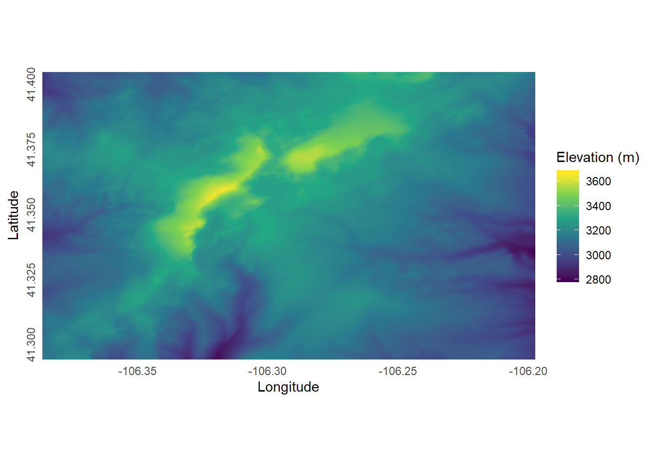
Alright, now let’s see what this clipped DEM looks like.

ggplot(snowy_df) +
  geom_raster(aes(x, y, fill = z)) +
  scale_fill_viridis_c() +
  labs(x = "Longitude",
    y = "Latitude",
    fill = "Elevation (m)") +
  coord_equal() +
  theme_minimal() +
  theme(axis.text.y = element_text(angle = 90, hjust = 0.43)) +
  scale_x_continuous(expand = c(0, 0)) +
  scale_y_continuous(expand = c(0, 0))

Nice. Now let’s see what the rayshader graphic looks like.

Dynamic visualization

This visual output from this render process can be pretty large (> 60 MB), so it may take a hot second to load.

#Convert the Snowy Range raster to a matrix.
snowy_mat = matrix(
  data = raster::extract(snowy, raster::extent(snowy),
  buffer = 1500),
  nrow = ncol(snowy),
  ncol = nrow(snowy)
  )

#Initialize some of the rayshader inputs.
z_scale <- 8 #Stretching out the elevations for a bit of visual appeal.
snowy_norm <- calculate_normal(snowy_mat, zscale = z_scale)
snowy_shadow <- ray_shade(snowy_mat, zscale = z_scale)
snowy_amb <- ambient_shade(snowy_mat, zscale = z_scale)

#Visualize!
snowy_mat %>%
  sphere_shade(
    zscale = z_scale,
    texture = "imhof4",
    normalvectors = snowy_norm) %>%
  add_shadow(snowy_shadow) %>%
  add_shadow(snowy_amb) %>%
  plot_3d(snowy_mat,
    zscale = z_scale,
    zoom = 0.5,
    baseshape = "circle")
#Capture the rgl output.
rglwidget(height = "600",
  elementId = "snowy-3d")