- Introduction
- Dialect comparison
- Importing data
- Dataframe-base data manipulations
- Globally remove NAs
- Interlude: Piping
- If-else conditional manipulations
- Multiple condition manipulations
- Filtering observations (rows)
- Column manipulation: Changing a column
- Interlude: Related tidyverse
mutatefunctions - Interlude: Dot (.) notation in the tidyverse
- Column manipulation: Adding columns
- Selecting variables (columns): Positive indexing
- Interlude: Infix operators
- Selecting variables (columns): Negative indexing
- Renaming variables (columns)
- Interlude: Back ticks
- Joining data
- Joining data: Full join
- Joining data: Inner join
- Joining data: Left join
- Joining data: Right join
- Interlude: Tidy data and why it is useful
- Data reshaping (pivoting): Observations to variables
- Data reshaping (pivoting): Variables to observations
- Iterators
- Split-apply-combine: Simple aggregations
- Split-apply-combine: More complicatated aggregations
- Appendix of other useful information
Synopsis: Below are a number of examples comparing different ways to use base R, the tidyverse, and data.table. These examples are meant to provide something of a Rosetta Stone (an incomplete comparison of the dialects, but good enough to start the deciphering process) for comparing some common tasks in R using the different dialects. The examples start fairly simply and get progressively harder. I provide some additional information along the way, in case folks are new to R or programming more generally.
Introduction
Welcome! If you use R you likely know there are different “flavors” (I’ll call them dialects or syntaxes) of the language that people use. Specifically, the common dialects are “base R”, the tidyverse, and data.table. Base R is what you get when you open up R for the first time, and was the only dialect for a long time. The tidyverse and data.table, in contrast, are add-ons (via packages) to the language. In my opinion, both add-on dialects drastically improve certain aspects of R, though there are definitely merits to coding only in base.
Some folks seem to prefer one coding style over another, but I think each dialect has it’s merits, and the use of a dialect depends on the problem at hand, as well as personal preference. For me, I just really like having different options that can solve different problems. The tidyverse, for example, emphasizes readability and flexibility, which is great when I need to write scaleable code that others can easily read. data.table, on the other hand, is lightening fast and very concise, so you can develop quickly and run super fast code, even when datasets get fairly large. Base R, however, is super stable, which may allow your code to withstand the tests of time for those longer-term projects. Base R is also closer to a “pure” programming language, meaning some of the base skills are more transferable to other languages.
Despite the benefits of each dialect, though, translating can sometimes be difficult. The intent of this post, then, is to provide a sense of how one might code the same task across dialects. These examples and translations are not meant to be exhaustive (there are many paths up this mountain). They’re probably not even best practice. But they are a way forward. And sometimes that is what is needed more than anything.
Libraries
Below are the librarries used to create this document. I’m letting knitr print the tidyverse messages to the page so you can see what exact packages are core to the tidyverse. Other packages I use a lot are broom (which I’ll use here; great for getting tidy synopses of model outputs) and lubridate (for working with dates and times in R).
library(magrittr) #Exports the special pipe we'll use, `%<>%`
library(data.table) #The data.table package
library(tidyverse) #Loads all the packages from the tidyverse
## -- Attaching packages ------------------------------------------------------------------ tidyverse 1.3.0 --## v ggplot2 3.2.1 v purrr 0.3.3
## v tibble 2.1.3 v dplyr 0.8.4
## v tidyr 1.0.2 v stringr 1.4.0
## v readr 1.3.1 v forcats 0.4.0## -- Conflicts --------------------------------------------------------------------- tidyverse_conflicts() --
## x dplyr::between() masks data.table::between()
## x tidyr::extract() masks magrittr::extract()
## x dplyr::filter() masks stats::filter()
## x dplyr::first() masks data.table::first()
## x dplyr::lag() masks stats::lag()
## x dplyr::last() masks data.table::last()
## x purrr::set_names() masks magrittr::set_names()
## x purrr::transpose() masks data.table::transpose()The data
For the sake of consistency, we’ll work with the CO2 dataset, which comes with R. Focusing mostly on just this one dataset will keep things simple.
#Load in the data
data("CO2")
In case you don’t have R open, the table below provides all the data, to help convey the structure of CO2.
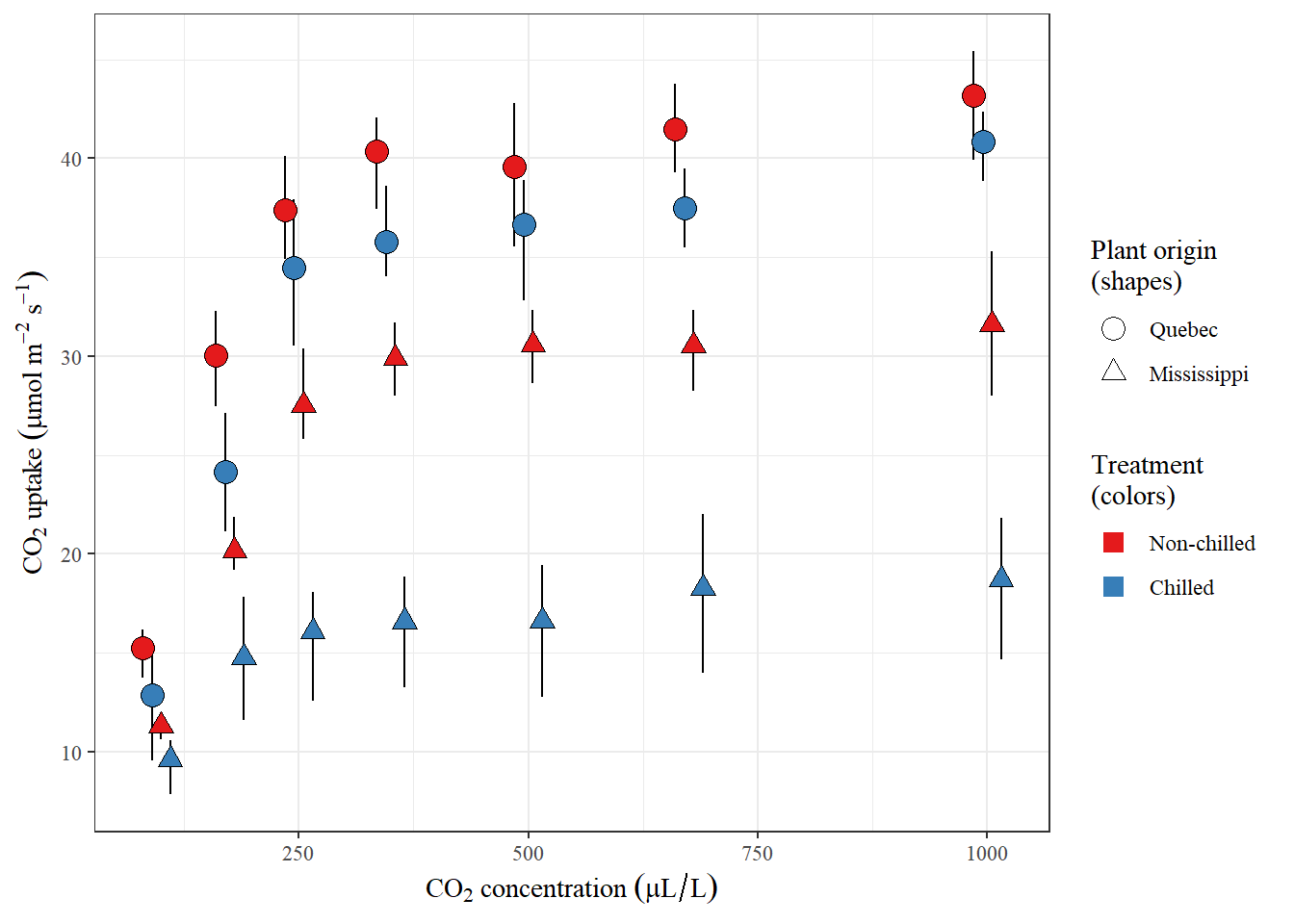
Below is a visual summary of the dataset (along with code), to help highlight the relationships between the different variables.
CO2 %>%
  #Summarise the data for easier plotting
  group_by(Type, Treatment, conc) %>%
  summarise(mean = mean(uptake),
    lo = quantile(uptake, probs = 0.975),
    hi = quantile(uptake, probs = 0.025)) %>%
  ungroup() %>%
  #Change the names to something a little nicer looking
  mutate(Treatment = fct_recode(Treatment, Chilled = "chilled",
    `Non-chilled` = "nonchilled")) %>%
  #Plot!
  ggplot(aes(conc, mean, fill = Treatment, group = interaction(conc, Treatment, Type))) +
  geom_errorbar(aes(ymax = hi, ymin = lo),
    width = 0,
    position = position_jitterdodge(jitter.width = 0, dodge.width = 40,
      seed = 20200120)) +
  geom_point(aes(shape = Type, size = Type),
    position = position_jitterdodge(jitter.width = 0, dodge.width = 40,
      seed = 20200120)) +
  labs(x = expression(CO[2]~concentration~(mu*L/L)),
    y = expression(CO[2]~uptake~(mu*mol~m^{-2}~s^{-1})),
    fill = "Treatment\n(colors)",
    shape = "Plant origin\n(shapes)",
    size = "Plant origin\n(shapes)") +
  theme_bw() +
  theme(text = element_text(family = "serif")) +
  scale_shape_manual(values = c(21, 24)) +
  scale_size_manual(values = c(4, 3)) +
  scale_fill_brewer(palette = "Set1") +
  guides(fill = guide_legend(override.aes = list(shape = 22, size = 4, stroke = NA)))
Figure 1: Figure: A visual summary of the CO2 data set. Error bars represent the 95th percentile of a given set of measurements, while the point (shape) is the mean. Note that CO2 concentrations are slightly jittered to improve visualization of the data by reducing overlap between points.
Dialect comparison
This post was largely inpsired by significant digit’s blog post, which provides an even longer comparison of base and tidyverse functions, but does not provide data.table alternatives.
The sections below are organized by similar tasks, getting progressively more difficult. In some cases I provide different versions of the same task, each with a slight twist. I also tried to keep each dialect in the same order for every task. In that context, each section contains color-coordinated base R code, tidyverse code, and data.table code that all do the same thing, but in their own way. You can click each code block to reveal the result of that block. Below are just some examples of what that interactivity looks like.
I should mention that I don’t use data.table much (one of the reasons I’m making this document – to get better at using and understanding the package), so some of that code may not always be very good. In fact, none of it may be very good, but it will get the job done, sooo…
This is a **base R** code block. Click this block to reveal the code result.## This is a base R result block. Click either this or the above block to hide the result.This is a **tidyverse** code block. Click this block to reveal the code result.## This is a tidyverse result block. Click either this or the above block to hide the result.This is a **data.table** code block. Click this block to reveal the result of this code.## This is a data.table result block. Click either this or the above block to hide the result.In some cases multiple examples of a tasks are provide. In other cases a paricular task cannot be easily performed using a given synax, so no example is provided.
Importing data
Reading in csv data
Importing data is a pretty basic task. Below are just a few examples of how we might import data from a csv file across dialects. For other ways of importing data, check out the appendix.
data_base <- read.csv("../../static/data/co2.csv", stringsAsFactors = FALSE)
head(data_base)
## Plant Type Treatment conc uptake
## 1 Qn1 Quebec nonchilled NA 16.0
## 2 Qn1 Quebec nonchilled 175 30.4
## 3 Qn1 Quebec nonchilled 250 34.8
## 4 Qn1 Quebec nonchilled 350 37.2
## 5 Qn1 Quebec nonchilled 500 35.3
## 6 Qn1 Quebec nonchilled 675 39.2data_tidy <- read_csv("../../static/data/co2.csv")
head(data_tidy)## # A tibble: 6 x 5
## Plant Type Treatment conc uptake
## <chr> <chr> <chr> <dbl> <dbl>
## 1 Qn1 Quebec nonchilled NA 16
## 2 Qn1 Quebec nonchilled 175 30.4
## 3 Qn1 Quebec nonchilled 250 34.8
## 4 Qn1 Quebec nonchilled 350 37.2
## 5 Qn1 Quebec nonchilled 500 35.3
## 6 Qn1 Quebec nonchilled 675 39.2data_dt <- fread("../../static/data/co2.csv")
head(data_dt)## Plant Type Treatment conc uptake
## 1: Qn1 Quebec nonchilled NA 16.0
## 2: Qn1 Quebec nonchilled 175 30.4
## 3: Qn1 Quebec nonchilled 250 34.8
## 4: Qn1 Quebec nonchilled 350 37.2
## 5: Qn1 Quebec nonchilled 500 35.3
## 6: Qn1 Quebec nonchilled 675 39.2Dataframe-base data manipulations
Dataframes are a key data type in R-based data analysis, so most of the this document will focus on manipulating this kind of data. However, some other types of manipulations are provided later in the document, which focus on combining dataframes and lists (dataframes are actually a kind of list).
Globally remove NAs
Certain kinds of analysis or workflows can’t handle NA values. Thus, it can sometimes be useful to remove all these values from a data frame.
data_base <- data_base[complete.cases(data_base), ]
head(data_base)
## Plant Type Treatment conc uptake
## 2 Qn1 Quebec nonchilled 175 30.4
## 3 Qn1 Quebec nonchilled 250 34.8
## 4 Qn1 Quebec nonchilled 350 37.2
## 5 Qn1 Quebec nonchilled 500 35.3
## 6 Qn1 Quebec nonchilled 675 39.2
## 7 Qn1 Quebec nonchilled 1000 39.7data_tidy <- drop_na(data_tidy)
head(data_tidy)## # A tibble: 6 x 5
## Plant Type Treatment conc uptake
## <chr> <chr> <chr> <dbl> <dbl>
## 1 Qn1 Quebec nonchilled 175 30.4
## 2 Qn1 Quebec nonchilled 250 34.8
## 3 Qn1 Quebec nonchilled 350 37.2
## 4 Qn1 Quebec nonchilled 500 35.3
## 5 Qn1 Quebec nonchilled 675 39.2
## 6 Qn1 Quebec nonchilled 1000 39.7data_dt <- na.omit(data_dt)
head(data_dt)## Plant Type Treatment conc uptake
## 1: Qn1 Quebec nonchilled 175 30.4
## 2: Qn1 Quebec nonchilled 250 34.8
## 3: Qn1 Quebec nonchilled 350 37.2
## 4: Qn1 Quebec nonchilled 500 35.3
## 5: Qn1 Quebec nonchilled 675 39.2
## 6: Qn1 Quebec nonchilled 1000 39.7Interlude: Piping
Piping (sometimes called chaining) is the action of taking initial or processed data and passing it to another function or variable. There are a couple of (overlapping) benefits to piping:
- Bloomin’ the onion: Base R code is often nested with the first function performed on some data inside of the nest and the last function on the outside. This nested structure is often difficult to read and understand. By reorganizing with pipes, starting with the data and passing the results to a series of functions, we can unnest our code, making data and actions performed on the data more obvious.
- Readability and intent: A typical consequence of reorganizing code using pipes is that the data and functions are now in a more logical order. This logical order improves code readability and the conveyence of intent, which is both good for future you (the person most likely to use your code again) and others potentially interested in using your code for their own work (such as a collaborator).
Here is a very contrived example of deeply nested code that gets the average values of two variables for two plants in the CO2 dataset. I’ve seen stuff like this in the wild, but there are much more efficient ways of doing this, even in base R (see the filtering, selecting, and aggregating examples).
as.data.frame(t(sapply(X = split(x = CO2[which(CO2$Plant %in% c("Mn2", "Mn3")), which(colnames(CO2) %in% c("conc", "uptake"))],
    f = CO2$Plant[which(CO2$Plant %in% c("Mn2", "Mn3"))],
    drop = TRUE),
  FUN = function(x) {apply(x, 2, mean)})))
## conc uptake
## Mn3 435 24.11429
## Mn2 435 27.34286Note that generating exactly the same results as those below would require some additional clean-up as the Plant names are now rownames and not their own column.
tidyverse
%>%: Used to pass either raw data or data resulting from a function to another function for addtional processing.%<>%: Not strictly part of the tidyverse, but I find it useful in some circumstances (and comes from the same package as%>%,magrittr). This operator basically replacesdata <- data %>% .... In otherwords, it just over-writes the current variable with whatever is returned from some functions/instructions that follow.
Below is a replacement for the nested base R code provided above:
CO2 %>%
  filter(Plant %in% c("Mn2", "Mn3")) %>% # Get the two plants we care about
  select(Plant, conc, uptake) %>% # Focus on the variable we want
  group_by(Plant) %>% # Seperate/group the analysis to focus on individual plants
  summarise_all(mean) # Get the means for conc and uptake
## # A tibble: 2 x 3
## Plant conc uptake
## <ord> <dbl> <dbl>
## 1 Mn3 435 24.1
## 2 Mn2 435 27.3Personally, I can read that much easer than the base code, though it requires some practice.
data.table
][: Effectively, pipes in data.table look as if you are connecting subsets of a dataframe. And really that’s what is happening, at some level.
Here is an example of using data.table’s pipes to, again, replace the nested base R code provided earlier:
CO2_dt <- CO2 # Copy to data to a format usable with data.table
setDT(CO2_dt) # Convert to data.table object
CO2_dt[Plant %in% c("Mn2", "Mn3"), # Get the plants we care about
  c("Plant", "conc", "uptake")  ][ # Select the variables of interest
  , lapply(.SD, mean), by = Plant] # List-apply the mean function using the .SD operator for each plant
## Plant conc uptake
## 1: Mn2 435 27.34286
## 2: Mn3 435 24.11429Basically, I could do in one call what might take multiple lines to do in base R or the tidyverse, and the result is run really fast. There are some extra things going on here, like the .SD object, but we can only cover so much… (to learn more about .SD in data.table, check out this vignette)
If-else conditional manipulations
If-else statements are useful when we’d like to evaluate a condition and return either option A or option B. We’ll use the vectorized form of if-else statements, for the sake of simplicity.
data_base$Treatment <- ifelse(data_base$Treatment == "non-chilled", "nonchilled", data_base$Treatment)
head(data_base)
## Plant Type Treatment conc uptake
## 2 Qn1 Quebec nonchilled 175 30.4
## 3 Qn1 Quebec nonchilled 250 34.8
## 4 Qn1 Quebec nonchilled 350 37.2
## 5 Qn1 Quebec nonchilled 500 35.3
## 6 Qn1 Quebec nonchilled 675 39.2
## 7 Qn1 Quebec nonchilled 1000 39.7data_tidy %<>% mutate(Treatment = if_else(Treatment == "non-chilled", "nonchilled", Treatment))
head(data_tidy)## # A tibble: 6 x 5
## Plant Type Treatment conc uptake
## <chr> <chr> <chr> <dbl> <dbl>
## 1 Qn1 Quebec nonchilled 175 30.4
## 2 Qn1 Quebec nonchilled 250 34.8
## 3 Qn1 Quebec nonchilled 350 37.2
## 4 Qn1 Quebec nonchilled 500 35.3
## 5 Qn1 Quebec nonchilled 675 39.2
## 6 Qn1 Quebec nonchilled 1000 39.7data_dt[, Treatment := ifelse(Treatment == "non-chilled", "nonchilled", Treatment)]
head(data_dt)## Plant Type Treatment conc uptake
## 1: Qn1 Quebec nonchilled 175 30.4
## 2: Qn1 Quebec nonchilled 250 34.8
## 3: Qn1 Quebec nonchilled 350 37.2
## 4: Qn1 Quebec nonchilled 500 35.3
## 5: Qn1 Quebec nonchilled 675 39.2
## 6: Qn1 Quebec nonchilled 1000 39.7Multiple condition manipulations
Sometimes it’s not enough to have only two conditions. In those cases we’d like to evaluate many possible outcomes. For those circumstances we can use the unvectorized switch() from base R, or the vectorized case_when() from the tidyverse. If you’d like to know more about vectorization, checkout this other post on the topic.
#Because `switch` is not vectorized, it's easier to use it in a stand alone function
# We can then use this function with an iterator (more on those later)
plant_switcher <- function(Plant) {
  switch(Plant,
         "Qn1" = "A nice plant",
         "Qn2" = "A lovely plant",
         "Qn3" = "A marvelous plant",
          Plant)}
data_base$Plant <- sapply(data_base$Plant, plant_switcher, USE.NAMES = FALSE)
head(data_base)
## Plant Type Treatment conc uptake
## 2 A nice plant Quebec nonchilled 175 30.4
## 3 A nice plant Quebec nonchilled 250 34.8
## 4 A nice plant Quebec nonchilled 350 37.2
## 5 A nice plant Quebec nonchilled 500 35.3
## 6 A nice plant Quebec nonchilled 675 39.2
## 7 A nice plant Quebec nonchilled 1000 39.7#`case_when` is already vectorized, so we don't need to use an iterator
data_tidy %<>% mutate(Plant = case_when(
Plant == "Qn1" ~ "A nice plant",
Plant == "Qn2" ~ "A lovely plant",
Plant == "Qn3" ~ "A marvelous plant",
#Default condition; just returns the current value of the Plant variable if the above
# conditions aren't met
TRUE ~ Plant))
head(data_tidy)## # A tibble: 6 x 5
## Plant Type Treatment conc uptake
## <chr> <chr> <chr> <dbl> <dbl>
## 1 A nice plant Quebec nonchilled 175 30.4
## 2 A nice plant Quebec nonchilled 250 34.8
## 3 A nice plant Quebec nonchilled 350 37.2
## 4 A nice plant Quebec nonchilled 500 35.3
## 5 A nice plant Quebec nonchilled 675 39.2
## 6 A nice plant Quebec nonchilled 1000 39.7plant_switcher <- function(Plant) {
switch(Plant,
"Qn1" = "A nice plant",
"Qn2" = "A lovely plant",
"Qn3" = "A marvelous plant",
Plant)}
data_dt[, Plant := plant_switcher(Plant), by = row.names(data_dt)]
head(data_dt)## Plant Type Treatment conc uptake
## 1: A nice plant Quebec nonchilled 175 30.4
## 2: A nice plant Quebec nonchilled 250 34.8
## 3: A nice plant Quebec nonchilled 350 37.2
## 4: A nice plant Quebec nonchilled 500 35.3
## 5: A nice plant Quebec nonchilled 675 39.2
## 6: A nice plant Quebec nonchilled 1000 39.7Filtering observations (rows)
Filtering involves returning only those rows of a dataframe that meet specific criteria. Boolean logic and indexing underlie this task, so be sure you understand how those two things can work together to filter in base R, as the same logic applies to the other two dialects.
#Option 1: Using boolean logic and indexing
data_base[data_base$Plant == "Mn1", ]
## Plant Type Treatment conc uptake
## 43 Mn1 Mississippi nonchilled 95 10.6
## 44 Mn1 Mississippi nonchilled 175 19.2
## 45 Mn1 Mississippi nonchilled 250 26.2
## 46 Mn1 Mississippi nonchilled 350 30.0
## 47 Mn1 Mississippi nonchilled 500 30.9
## 48 Mn1 Mississippi nonchilled 675 32.4
## 49 Mn1 Mississippi nonchilled 1000 35.5#Option 2: Using `subset()`
subset(data_base, Plant == "Mn1")## Plant Type Treatment conc uptake
## 43 Mn1 Mississippi nonchilled 95 10.6
## 44 Mn1 Mississippi nonchilled 175 19.2
## 45 Mn1 Mississippi nonchilled 250 26.2
## 46 Mn1 Mississippi nonchilled 350 30.0
## 47 Mn1 Mississippi nonchilled 500 30.9
## 48 Mn1 Mississippi nonchilled 675 32.4
## 49 Mn1 Mississippi nonchilled 1000 35.5filter(data_tidy, Plant == "Mn1")## # A tibble: 7 x 5
## Plant Type Treatment conc uptake
## <chr> <chr> <chr> <dbl> <dbl>
## 1 Mn1 Mississippi nonchilled 95 10.6
## 2 Mn1 Mississippi nonchilled 175 19.2
## 3 Mn1 Mississippi nonchilled 250 26.2
## 4 Mn1 Mississippi nonchilled 350 30
## 5 Mn1 Mississippi nonchilled 500 30.9
## 6 Mn1 Mississippi nonchilled 675 32.4
## 7 Mn1 Mississippi nonchilled 1000 35.5data_dt[Plant == "Mn1"]## Plant Type Treatment conc uptake
## 1: Mn1 Mississippi nonchilled 95 10.6
## 2: Mn1 Mississippi nonchilled 175 19.2
## 3: Mn1 Mississippi nonchilled 250 26.2
## 4: Mn1 Mississippi nonchilled 350 30.0
## 5: Mn1 Mississippi nonchilled 500 30.9
## 6: Mn1 Mississippi nonchilled 675 32.4
## 7: Mn1 Mississippi nonchilled 1000 35.5Column manipulation: Changing a column
Sometimes you need to change the values of a variable that already exist. In this example we’ll convert the concentration of CO2 from mL/L to L/L.
data_base$conc <- data_base$conc / 1000
head(data_base)
## Plant Type Treatment conc uptake
## 2 A nice plant Quebec nonchilled 0.175 30.4
## 3 A nice plant Quebec nonchilled 0.250 34.8
## 4 A nice plant Quebec nonchilled 0.350 37.2
## 5 A nice plant Quebec nonchilled 0.500 35.3
## 6 A nice plant Quebec nonchilled 0.675 39.2
## 7 A nice plant Quebec nonchilled 1.000 39.7data_tidy %<>% mutate(conc = conc / 1000)
head(data_tidy)## # A tibble: 6 x 5
## Plant Type Treatment conc uptake
## <chr> <chr> <chr> <dbl> <dbl>
## 1 A nice plant Quebec nonchilled 0.175 30.4
## 2 A nice plant Quebec nonchilled 0.25 34.8
## 3 A nice plant Quebec nonchilled 0.35 37.2
## 4 A nice plant Quebec nonchilled 0.5 35.3
## 5 A nice plant Quebec nonchilled 0.675 39.2
## 6 A nice plant Quebec nonchilled 1 39.7data_dt[, conc := conc / 1000]
head(data_dt)## Plant Type Treatment conc uptake
## 1: A nice plant Quebec nonchilled 0.175 30.4
## 2: A nice plant Quebec nonchilled 0.250 34.8
## 3: A nice plant Quebec nonchilled 0.350 37.2
## 4: A nice plant Quebec nonchilled 0.500 35.3
## 5: A nice plant Quebec nonchilled 0.675 39.2
## 6: A nice plant Quebec nonchilled 1.000 39.7Interlude: Dot (.) notation in the tidyverse
Dot notation is used to symbolically pass the result of a pipe to another function. This passing can either be explicit or implicit. One benefit of dot notation is that we do not have to explictly name intermediate objects passed from one function to another function during piping. The downside of this syntax is that the learning curve is steep. However, once you learn this convention, it can make your coding style much more flexible, meaning, code reusability increases.
An implict example of using dot notation:
CO2 %>% mutate(new_column = "data in new col") %>% head()## # A tibble: 6 x 6
## Plant Type Treatment conc uptake new_column
## <chr> <chr> <chr> <dbl> <dbl> <chr>
## 1 Qn1 Quebec nonchilled 95 16 data in new col
## 2 Qn1 Quebec nonchilled 175 30.4 data in new col
## 3 Qn1 Quebec nonchilled 250 34.8 data in new col
## 4 Qn1 Quebec nonchilled 350 37.2 data in new col
## 5 Qn1 Quebec nonchilled 500 35.3 data in new col
## 6 Qn1 Quebec nonchilled 675 39.2 data in new colAn explicit example of using dot notation
#Note that '.data' is the name of the first argument of the mutate function.
CO2 %>% mutate(.data = ., new_column = "data in new col") %>% head()
## # A tibble: 6 x 6
## Plant Type Treatment conc uptake new_column
## <chr> <chr> <chr> <dbl> <dbl> <chr>
## 1 Qn1 Quebec nonchilled 95 16 data in new col
## 2 Qn1 Quebec nonchilled 175 30.4 data in new col
## 3 Qn1 Quebec nonchilled 250 34.8 data in new col
## 4 Qn1 Quebec nonchilled 350 37.2 data in new col
## 5 Qn1 Quebec nonchilled 500 35.3 data in new col
## 6 Qn1 Quebec nonchilled 675 39.2 data in new colIn the example below, the . no longer represents the dataframe being passed to mutate_at, but the individual columns being passed to the mean function. This the meaning of . depends on context.
mutate_at(data_tidy, vars(uptake, conc), list(mean = ~mean(.))) %>% head()## # A tibble: 6 x 7
## Plant Type Treatment conc uptake uptake_mean conc_mean
## <chr> <chr> <chr> <dbl> <dbl> <dbl> <dbl>
## 1 A nice plant Quebec nonchilled 0.175 30.4 27.3 0.304
## 2 A nice plant Quebec nonchilled 0.25 34.8 27.3 0.304
## 3 A nice plant Quebec nonchilled 0.35 37.2 27.3 0.304
## 4 A nice plant Quebec nonchilled 0.5 35.3 27.3 0.304
## 5 A nice plant Quebec nonchilled 0.675 39.2 27.3 0.304
## 6 A nice plant Quebec nonchilled 1 39.7 27.3 0.304Column manipulation: Adding columns
Sometimes we need to make a new variable, which might be some new information, or the combination of other variables. Here, we’ll scale the uptake and conc variables so that their values are roughly standard normal (normally distributed with a mean of zero and a standard deviation of one).
data_base$conc_scaled <- scale(data_base$conc)
data_base$uptake_scaled <- scale(data_base$uptake)
head(data_base)
## Plant Type Treatment conc uptake conc_scaled uptake_scaled
## 2 A nice plant Quebec nonchilled 0.175 30.4 -0.10883975 0.2823498
## 3 A nice plant Quebec nonchilled 0.250 34.8 -0.04534883 0.6894328
## 4 A nice plant Quebec nonchilled 0.350 37.2 0.03930572 0.9114781
## 5 A nice plant Quebec nonchilled 0.500 35.3 0.16628755 0.7356923
## 6 A nice plant Quebec nonchilled 0.675 39.2 0.31443302 1.0965159
## 7 A nice plant Quebec nonchilled 1.000 39.7 0.58956032 1.1427753data_tidy %<>% mutate_at(vars(conc, uptake), list(scaled = ~scale(.)[, 1]))
head(data_tidy)## # A tibble: 6 x 7
## Plant Type Treatment conc uptake conc_scaled uptake_scaled
## <chr> <chr> <chr> <dbl> <dbl> <dbl> <dbl>
## 1 A nice plant Quebec nonchilled 0.175 30.4 -0.109 0.282
## 2 A nice plant Quebec nonchilled 0.25 34.8 -0.0453 0.689
## 3 A nice plant Quebec nonchilled 0.35 37.2 0.0393 0.911
## 4 A nice plant Quebec nonchilled 0.5 35.3 0.166 0.736
## 5 A nice plant Quebec nonchilled 0.675 39.2 0.314 1.10
## 6 A nice plant Quebec nonchilled 1 39.7 0.590 1.14data_dt[, conc_scaled := scale(conc)]
data_dt[, uptake_scaled := scale(uptake)]
head(data_dt)## Plant Type Treatment conc uptake conc_scaled uptake_scaled
## 1: A nice plant Quebec nonchilled 0.175 30.4 -0.10883975 0.2823498
## 2: A nice plant Quebec nonchilled 0.250 34.8 -0.04534883 0.6894328
## 3: A nice plant Quebec nonchilled 0.350 37.2 0.03930572 0.9114781
## 4: A nice plant Quebec nonchilled 0.500 35.3 0.16628755 0.7356923
## 5: A nice plant Quebec nonchilled 0.675 39.2 0.31443302 1.0965159
## 6: A nice plant Quebec nonchilled 1.000 39.7 0.58956032 1.1427753Selecting variables (columns): Positive indexing
Sometimes we don’t need every bit of information for a given analysis and instead just need to focus on a few variables. One way of selecting variables is to name all the variables we’d like to include in our analysis.
data_base <- data_base[, c("Plant", "Type", "Treatment", "conc", "uptake", "conc_scaled")]
head(data_base)
## Plant Type Treatment conc uptake conc_scaled
## 2 A nice plant Quebec nonchilled 0.175 30.4 -0.10883975
## 3 A nice plant Quebec nonchilled 0.250 34.8 -0.04534883
## 4 A nice plant Quebec nonchilled 0.350 37.2 0.03930572
## 5 A nice plant Quebec nonchilled 0.500 35.3 0.16628755
## 6 A nice plant Quebec nonchilled 0.675 39.2 0.31443302
## 7 A nice plant Quebec nonchilled 1.000 39.7 0.58956032data_tidy %<>% select(Plant, Type, Treatment, conc, uptake, conc_scaled)
head(data_tidy)## # A tibble: 6 x 6
## Plant Type Treatment conc uptake conc_scaled
## <chr> <chr> <chr> <dbl> <dbl> <dbl>
## 1 A nice plant Quebec nonchilled 0.175 30.4 -0.109
## 2 A nice plant Quebec nonchilled 0.25 34.8 -0.0453
## 3 A nice plant Quebec nonchilled 0.35 37.2 0.0393
## 4 A nice plant Quebec nonchilled 0.5 35.3 0.166
## 5 A nice plant Quebec nonchilled 0.675 39.2 0.314
## 6 A nice plant Quebec nonchilled 1 39.7 0.590data_dt <- data_dt[, c("Plant", "Type", "Treatment", "conc", "uptake", "conc_scaled") , with = FALSE]
head(data_dt)## Plant Type Treatment conc uptake conc_scaled
## 1: A nice plant Quebec nonchilled 0.175 30.4 -0.10883975
## 2: A nice plant Quebec nonchilled 0.250 34.8 -0.04534883
## 3: A nice plant Quebec nonchilled 0.350 37.2 0.03930572
## 4: A nice plant Quebec nonchilled 0.500 35.3 0.16628755
## 5: A nice plant Quebec nonchilled 0.675 39.2 0.31443302
## 6: A nice plant Quebec nonchilled 1.000 39.7 0.58956032Interlude: Infix operators
Infix operators are functions that have two arguments, a left-hand side and are right-hand side. They are different from regular operators in that they are not usually surrounded by parentheses. Really common infix operators are the arithmetic operators, such as +, -, *, /. However, there are others, like the pipe used in the tidyverse, %>%, and the matching operator, %in%, which returns TRUE and FALSE values based on whether or not elements in the left-hand side exist in the right-hand side. For example:
c('Hello', 'world', '!') %in% c('world', 'Hello')## [1] TRUE TRUE FALSEThis kind of thing can be useful for indexing parts of a vector, dataframe, etc., in which we are only interested in some parts of those data objects:
hello_world <- c('Hello', 'world', '!', 'extra', 'text')
hello_world[hello_world %in% c('Hello', 'words', 'not', 'in', 'vector', 'world')]
## [1] "Hello" "world"Infix operators can also be turned into regular functions using backticks. For example:
`+`(2, 3) # Just like saying: 2 + 3## [1] 5Selecting variables (columns): Negative indexing
Sometimes we want most of our variables, getting rid of only a few. It can be super inefficient to use positive selection/indexing to do that, especially if we have lots of variables. Instead, it might make more sense to select which variables we don’t want.
#Option 1: Using the negation operator, `!` (pronounced "bang" or "bang operator")
data_base <- data_base[!(names(data_base) %in% "conc_scaled")]
head(data_base)
## Plant Type Treatment conc uptake
## 2 A nice plant Quebec nonchilled 0.175 30.4
## 3 A nice plant Quebec nonchilled 0.250 34.8
## 4 A nice plant Quebec nonchilled 0.350 37.2
## 5 A nice plant Quebec nonchilled 0.500 35.3
## 6 A nice plant Quebec nonchilled 0.675 39.2
## 7 A nice plant Quebec nonchilled 1.000 39.7#Option 2: Using `subset()`
data_base <- subset(data_base, TRUE, select = -conc_scaled)
head(data_base)## Plant Type Treatment conc uptake
## 2 A nice plant Quebec nonchilled 0.175 30.4
## 3 A nice plant Quebec nonchilled 0.250 34.8
## 4 A nice plant Quebec nonchilled 0.350 37.2
## 5 A nice plant Quebec nonchilled 0.500 35.3
## 6 A nice plant Quebec nonchilled 0.675 39.2
## 7 A nice plant Quebec nonchilled 1.000 39.7#Scenario 1: Removing a single variable
data_tidy %<>% select(-conc_scaled)
head(data_tidy)## # A tibble: 6 x 5
## Plant Type Treatment conc uptake
## <chr> <chr> <chr> <dbl> <dbl>
## 1 A nice plant Quebec nonchilled 0.175 30.4
## 2 A nice plant Quebec nonchilled 0.25 34.8
## 3 A nice plant Quebec nonchilled 0.35 37.2
## 4 A nice plant Quebec nonchilled 0.5 35.3
## 5 A nice plant Quebec nonchilled 0.675 39.2
## 6 A nice plant Quebec nonchilled 1 39.7#Scenario 2: Removing multiple variables
data_tidy %<>% select(-c(conc_scaled, uptake_scaled))
head(data_tidy)## # A tibble: 6 x 5
## Plant Type Treatment conc uptake
## <chr> <chr> <chr> <dbl> <dbl>
## 1 A nice plant Quebec nonchilled 0.175 30.4
## 2 A nice plant Quebec nonchilled 0.25 34.8
## 3 A nice plant Quebec nonchilled 0.35 37.2
## 4 A nice plant Quebec nonchilled 0.5 35.3
## 5 A nice plant Quebec nonchilled 0.675 39.2
## 6 A nice plant Quebec nonchilled 1 39.7data_dt <- data_dt[, !"conc_scaled", with = FALSE]
head(data_dt)## Plant Type Treatment conc uptake
## 1: A nice plant Quebec nonchilled 0.175 30.4
## 2: A nice plant Quebec nonchilled 0.250 34.8
## 3: A nice plant Quebec nonchilled 0.350 37.2
## 4: A nice plant Quebec nonchilled 0.500 35.3
## 5: A nice plant Quebec nonchilled 0.675 39.2
## 6: A nice plant Quebec nonchilled 1.000 39.7Renaming variables (columns)
Sometimes variable names are too long, not very informative, or need to be named something specific for a workflow. Below are some examples of renaming variables.
colnames(data_base)[colnames(data_tidy) == "conc"] <- "co2_concentration"
colnames(data_base)[colnames(data_tidy) == "uptake"] <- "co2_uptake"
head(data_base)
## Plant Type Treatment co2_concentration co2_uptake
## 2 A nice plant Quebec nonchilled 0.175 30.4
## 3 A nice plant Quebec nonchilled 0.250 34.8
## 4 A nice plant Quebec nonchilled 0.350 37.2
## 5 A nice plant Quebec nonchilled 0.500 35.3
## 6 A nice plant Quebec nonchilled 0.675 39.2
## 7 A nice plant Quebec nonchilled 1.000 39.7data_tidy %<>% rename(co2_concentration = conc, co2_uptake = uptake)
head(data_tidy)## # A tibble: 6 x 5
## Plant Type Treatment co2_concentration co2_uptake
## <chr> <chr> <chr> <dbl> <dbl>
## 1 A nice plant Quebec nonchilled 0.175 30.4
## 2 A nice plant Quebec nonchilled 0.25 34.8
## 3 A nice plant Quebec nonchilled 0.35 37.2
## 4 A nice plant Quebec nonchilled 0.5 35.3
## 5 A nice plant Quebec nonchilled 0.675 39.2
## 6 A nice plant Quebec nonchilled 1 39.7setnames(data_dt, c('conc', 'uptake'), c('co2_concentration', 'co2_uptake'))
head(data_dt)## Plant Type Treatment co2_concentration co2_uptake
## 1: A nice plant Quebec nonchilled 0.175 30.4
## 2: A nice plant Quebec nonchilled 0.250 34.8
## 3: A nice plant Quebec nonchilled 0.350 37.2
## 4: A nice plant Quebec nonchilled 0.500 35.3
## 5: A nice plant Quebec nonchilled 0.675 39.2
## 6: A nice plant Quebec nonchilled 1.000 39.7Interlude: Back ticks
I’ve already mentioned back ticks, but only in reference to infix operators. However, back ticks can do other stuff. For example, if you want an R object start with a number or have spaces, then back ticks can be really useful. For example:
`2_dataframes_combined` <- bind_rows(data_base, data_tidy)
head(`2_dataframes_combined`)
## Plant Type Treatment co2_concentration co2_uptake
## 1 A nice plant Quebec nonchilled 0.175 30.4
## 2 A nice plant Quebec nonchilled 0.250 34.8
## 3 A nice plant Quebec nonchilled 0.350 37.2
## 4 A nice plant Quebec nonchilled 0.500 35.3
## 5 A nice plant Quebec nonchilled 0.675 39.2
## 6 A nice plant Quebec nonchilled 1.000 39.7Or:
`2 more dataframes combined` <- bind_rows(data_base, data_dt)
head(`2 more dataframes combined`)
## Plant Type Treatment co2_concentration co2_uptake
## 1 A nice plant Quebec nonchilled 0.175 30.4
## 2 A nice plant Quebec nonchilled 0.250 34.8
## 3 A nice plant Quebec nonchilled 0.350 37.2
## 4 A nice plant Quebec nonchilled 0.500 35.3
## 5 A nice plant Quebec nonchilled 0.675 39.2
## 6 A nice plant Quebec nonchilled 1.000 39.7Similarly, one can use back ticks to name columns in a dataframe (useful for passing label expressions to ggplot2). Example:
`2 more dataframes combined` %>%
  rename(`conc <L/L CO2>` = co2_concentration) %>%
  head()
## Plant Type Treatment conc <L/L CO2> co2_uptake
## 1 A nice plant Quebec nonchilled 0.175 30.4
## 2 A nice plant Quebec nonchilled 0.250 34.8
## 3 A nice plant Quebec nonchilled 0.350 37.2
## 4 A nice plant Quebec nonchilled 0.500 35.3
## 5 A nice plant Quebec nonchilled 0.675 39.2
## 6 A nice plant Quebec nonchilled 1.000 39.7This kind of syntax can be useful for including additional information in column names (attributes could be used, though that might be less obvious), or for use with math plotting. I’ll leave you all to find examples of thatkind of thing.
Joining data
There are many times in which related data are in different data files, but it is the combination of those data files that is really useful (e.g., one file contains metadata). To combine these disperate, but related data, we use joins. To make the process of joining data more concrete, we’ll make and use some simpler data than we’ve been using.
#base's dataframes
lhs_base = data.frame(LETTERS = LETTERS[1:3],
  numbers = 1:3,
  stringsAsFactors = FALSE)
rhs_base = data.frame(numbers = 3:4,
  letters = letters[3:4],
  stringsAsFactors = FALSE)

#tidyverse's tibbles
lhs_tidy = tibble(LETTERS = LETTERS[1:3],
  numbers = 1:3)
rhs_tidy = tibble(numbers = 3:4,
  letters = letters[3:4])

#data.table's datatables
lhs_dt = data.table(LETTERS = LETTERS[1:3],
  numbers = 1:3)
rhs_dt = data.table(numbers = 3:4,
  letters = letters[3:4])
Here’s what those data look like (using the tidyverse data as an example):
lhs_tidy; rhs_tidy## # A tibble: 3 x 2
## LETTERS numbers
## <chr> <int>
## 1 A 1
## 2 B 2
## 3 C 3## # A tibble: 2 x 2
## numbers letters
## <int> <chr>
## 1 3 c
## 2 4 dJoining data: Full join
In this version of joining data, all data is kept, no matter its source. This can sometimes result in a lot of NAs, where there was no overlapping information between data sets.
In the examples below I do not specify a by argument as the two dataframes being joined share the same variable names, thus the argument is implicit. Basically, this is a really simplified example of how these functions can be used.
merge(lhs_base, rhs_base, all = TRUE)## numbers LETTERS letters
## 1 1 A <NA>
## 2 2 B <NA>
## 3 3 C c
## 4 4 <NA> dfull_join(lhs_tidy, rhs_tidy)## # A tibble: 4 x 3
## LETTERS numbers letters
## <chr> <int> <chr>
## 1 A 1 <NA>
## 2 B 2 <NA>
## 3 C 3 c
## 4 <NA> 4 dmerge(lhs_dt, rhs_dt, all = TRUE)## numbers LETTERS letters
## 1: 1 A <NA>
## 2: 2 B <NA>
## 3: 3 C c
## 4: 4 <NA> dJoining data: Inner join
This version of joining keeps only observations present in both datasets. Again, the by argument is implictly handled.
merge(lhs_base, rhs_base)## numbers LETTERS letters
## 1 3 C cinner_join(lhs_tidy, rhs_tidy)## # A tibble: 1 x 3
## LETTERS numbers letters
## <chr> <int> <chr>
## 1 C 3 cmerge(lhs_dt, rhs_dt)## numbers LETTERS letters
## 1: 3 C cJoining data: Left join
Left joins will keep all the data from the first (left) left_join/merge argument, but will drop data from the second data set (right-hand side).
merge(lhs_base, rhs_base, all.x = TRUE)## numbers LETTERS letters
## 1 1 A <NA>
## 2 2 B <NA>
## 3 3 C cleft_join(lhs_tidy, rhs_tidy)## # A tibble: 3 x 3
## LETTERS numbers letters
## <chr> <int> <chr>
## 1 A 1 <NA>
## 2 B 2 <NA>
## 3 C 3 cmerge(lhs_dt, rhs_dt, all.x = TRUE)## numbers LETTERS letters
## 1: 1 A <NA>
## 2: 2 B <NA>
## 3: 3 C cJoining data: Right join
Same-same, but emphasizing the second dataframe passed to the function.
merge(lhs_base, rhs_base, all.y = TRUE)## numbers LETTERS letters
## 1 3 C c
## 2 4 <NA> dright_join(lhs_tidy, rhs_tidy)## # A tibble: 2 x 3
## LETTERS numbers letters
## <chr> <int> <chr>
## 1 C 3 c
## 2 <NA> 4 dmerge(lhs_dt, rhs_dt, all.y = TRUE)## numbers LETTERS letters
## 1: 3 C c
## 2: 4 <NA> dInterlude: Tidy data and why it is useful
Tidy data are generally rectangular data (e.g., a dataframe) where every row is an observation, every column is a variable, and every cell has a value. That might not sound very profound, but once you get used to working with tidy data programmatically, the benefits of this organizational strategy become pretty obvious. But what does untidy vs tidy data look like?
Here is an example of untidy data (this is actually reasonably tidy compared to a lot of “wild” data, but I needed something simple):
## # A tibble: 5 x 4
##   group    id time_point  mass
##   <dbl> <dbl>      <dbl> <dbl>
## 1     1   543          1  12.3
## 2    NA    NA          2  23.8
## 3    NA    23          1  28.9
## 4    NA    NA          2  18.3
## 5    NA    56          1  43
In the above table, group 1 (first column) implicitly applies to all the observations while the first id (second column) applies to the top 2 rows, and the second id applies to the bottom two rows. For some things this form is fine, but what if we need to start conditionally manipulating values. For example, what if we needed to add an offset to ever mass value for id 23? For small data sets, we could do this by hand in excel or a text editor (though that’s not a very reproducible solution), but for larger data sets (thousands of rows), we would have no easy way of tracking which observations are associated with id 23. Thus, tidy data uses redundancy to help as track the relationships between observations and variables.
The same data, but tidy:
##    group  id time_point mass
## 1:     1 543          1 12.3
## 2:     1 543          2 23.8
## 3:     1  23          1 28.9
## 4:     1  23          2 18.3
## 5:     1  56          1 43.0
One question we might ask is: What makes something an observation vs a variable? The answer to that issue depends on the larger questions being asked by the analysis and over all study. And because those bigger questions can change as we learn more about our data, we need to be able to change how observations and variables are treated in our data set. This process of manipulation is often called pivoting, which is discussed below.
For more on tidy data, check out the tidy data chapter in the R for Data Science book.
Data reshaping (pivoting): Observations to variables
In my experience, base R doesn’t have great reshaping resources, so I’m just going to avoid base for these reshaping examples.
From our tidy data example above, let’s say we want to turn time points from an observation to a variable. Here’ we’ll do that by “widening” our data such that
tidy_data %<>%
  pivot_wider(names_from = time_point,
    names_prefix = "time_point_",
    values_from = mass)
tidy_data
## # A tibble: 3 x 4
## group id time_point_1 time_point_2
## <dbl> <dbl> <dbl> <dbl>
## 1 1 543 12.3 23.8
## 2 1 23 28.9 18.3
## 3 1 56 43 NA#Prepend column name to ensure we can track source variable
dt_data[, time_point := paste("time_point", time_point, sep ="_")]
dt_data <- dcast(dt_data,
group + id ~ "time_point" + time_point,
value.var = "mass")
dt_data## group id time_point_1 time_point_2
## 1: 1 23 28.9 18.3
## 2: 1 56 43.0 NA
## 3: 1 543 12.3 23.8Notice that the last observation (id: 56) had no second time_point value, so it was provided a value of NA.
Data reshaping (pivoting): Variables to observations
Sometimes we want variables to become observations. This “lengthens” our data. In this example we’ll convert the “wide” data above, back into its original shape.
#pivot_longer
tidy_data %<>%
  pivot_longer(time_point_1:time_point_2,
    names_to = "time_point",
    names_prefix = "time_point_") %>%
  mutate(time_point = as.numeric(time_point))
tidy_data
## # A tibble: 6 x 4
## group id time_point value
## <dbl> <dbl> <dbl> <dbl>
## 1 1 543 1 12.3
## 2 1 543 2 23.8
## 3 1 23 1 28.9
## 4 1 23 2 18.3
## 5 1 56 1 43
## 6 1 56 2 NAdt_data <- melt(dt_data,
id_vars = "id",
measure.vars = c("time_point_1", "time_point_2"),
variable.name = "time_point")
dt_data[, time_point := as.numeric(gsub("time_point_", "", time_point))]
dt_data## group id time_point value
## 1: 1 23 1 28.9
## 2: 1 56 1 43.0
## 3: 1 543 1 12.3
## 4: 1 23 2 18.3
## 5: 1 56 2 NA
## 6: 1 543 2 23.8Notice that the NA value is now in our reshaped data. This kind of pivot wider-longer workflow can actually be really useful for identifying missing data or data combinations. It can also be useful as a placeholder for use in visualization software, like ggplot2.
Iterators
One nice thing about R is that it is largely a vectorized language, meaning we don’t have to explicity tell R to how to do something like:
c(2, 3) + c(3, 6)## [1] 5 9That is, R just knows that we want to loop through each paired value in the numeric vectors. However, that kind of vectorization is not always possible, in which case we need to explicitly iterate through our data somehow. In that context, we have two general kinds of iterator we can use: imperative and functional. We’ll focus on for loops as an example of imperative iteration. Functional iterators are very similar to their imperative counter-parts, but tend to be more scalable and flexible in how they operate, which is great for creating generalizable code that we can use over and over again.
Imperitive programming and the for loop
Loops are pretty fundamental to most (all?) contemporary programming languages, so there are not syntactical replacements for them (as far as I know). Thus the examples below simply provide some examples of using for loops in R to iterate through different data types.
Iterating over a vector:
some_letters <- letters[10:15]
some_letters
## [1] "j" "k" "l" "m" "n" "o"for(i in 1:length(some_letters)) {
cat(some_letters[i]) #Print a letter
cat("\n") #Tells R to print an empty line so they aren't all on one line
}## j
## k
## l
## m
## n
## oBonus question: Why do I need to use cat (or print) inside a for loop when I, for example, can simply type some_letters outside the loop and see the result printed to the console?
Iterating over the rows of a dataframe (and printing them):
for(row in 1:nrow(base_data)) {
  print(base_data[row, ])
  cat("\n")
}
## group id time_point mass
## 1 1 543 1 12.3
##
## group id time_point mass
## 2 1 543 2 23.8
##
## group id time_point mass
## 3 1 23 1 28.9
##
## group id time_point mass
## 4 1 23 2 18.3
##
## group id time_point mass
## 5 1 56 1 43Iterate over the columns of a dataframe (and print them):
for(column in 1:ncol(base_data)) {
  print(base_data[column])
  cat("\n")
}
## group
## 1 1
## 2 1
## 3 1
## 4 1
## 5 1
##
## id
## 1 543
## 2 543
## 3 23
## 4 23
## 5 56
##
## time_point
## 1 1
## 2 2
## 3 1
## 4 2
## 5 1
##
## mass
## 1 12.3
## 2 23.8
## 3 28.9
## 4 18.3
## 5 43.0For loops do not have to include only a single set of iterations, however. The example below highlights how we can nest loops by iterating over the different dimensions of a dataframe.
To help clarify how the column and row variables change over each iteration, I’ve added some extra formatting bits that track the variables. In this case column represents the “outer” loop and row represents in the “inner” loop.
for(column in 1:ncol(base_data)) {
  cat(paste0("[col: ", column, "]: New loop (", colnames(base_data)[column], ")"))
  cat("\n")
  for(row in 1:nrow(base_data)) {
    base_data[row, column] %>%
      paste0("[row: ", row, "]: ", .) %>%
      cat()
      cat("\n")
  }
  cat("\n") #Prints a new line between "inner" loops to help visualize the start/end of an iteration
}
## [col: 1]: New loop (group)
## [row: 1]: 1
## [row: 2]: 1
## [row: 3]: 1
## [row: 4]: 1
## [row: 5]: 1
##
## [col: 2]: New loop (id)
## [row: 1]: 543
## [row: 2]: 543
## [row: 3]: 23
## [row: 4]: 23
## [row: 5]: 56
##
## [col: 3]: New loop (time_point)
## [row: 1]: 1
## [row: 2]: 2
## [row: 3]: 1
## [row: 4]: 2
## [row: 5]: 1
##
## [col: 4]: New loop (mass)
## [row: 1]: 12.3
## [row: 2]: 23.8
## [row: 3]: 28.9
## [row: 4]: 18.3
## [row: 5]: 43A more suscinct version of the above loop that will just print out the numbers:
for(column in 1:ncol(base_data)) {
  for(row in 1:nrow(base_data)) {
    print(as.numeric(base_data[row, column]))
  }
}
We’re also not stuck with fixed values for our indeces when using for loops. That is, every iteration is an opportunity to change our indices for some purpose. For example, below is some code for making a random 3 x 3 upper triangular correlation matrix:
#Initialize the matrix
mat <- matrix(rep(0.0, times = 9), nrow = 3)
mat
## [,1] [,2] [,3]
## [1,] 0 0 0
## [2,] 0 0 0
## [3,] 0 0 0#Iterate over the matrix, adding the non-zero randome bits
for(n in 1:nrow(mat)) {
for(m in n:ncol(mat)) { #Note that we use "n" to start our iteration
if(n == m) {
mat[n, m] <- 1.0 #Ensures diagonal values are always equal to 1
} else {
mat[n, m] <- runif(1, -1, 1) #Random assignment of a value between -1 and 1
}
}
}
mat## [,1] [,2] [,3]
## [1,] 1 -0.938238 0.6599101
## [2,] 0 1.000000 0.5729254
## [3,] 0 0.000000 1.0000000Above, the first iteration of the inner loop we are focused on row 1, columns 1 to 3. In the second loop, column 2 and rows 2 to 3. In the final iteration we focus only on row 3, column 3.
Functional programming iterators (an alternative to imperative loops)
Functional iterators implictly perform some of the same actions as for loops, but usually with some extra bells and whistles. By themselves these functions are not usually that interesting, but when combined with other functions and workflows (e.g., the split-apply-combine method talked about in the next section) they can become real powerhouses.
In the case of base R, these iterators take the form of the *apply family, which include functions like apply(), lapply() (“list” apply), sapply() (“simplified” apply), etc. Personally, I find these functions very unintuitive, so I’m only going to provde an example of sapply.
For the tidyverse, most iterators are contained in the purrr package. The most important set of functional iterators in that package are the map family of functions.
As far as I can tell, the data.table package is really meant for workin with tidy, 2D data (columns and rows), so we’ll withhold the use of iteration until the next section.
Functional iteration can be kind of confusing, so we’ll keep it simple and brief. Just know that this stuff takes practice, so don’t worry if it doesn’t “click” at first. Just keep at it. In the examples below we’ll use the following function to test if a number is “big” or “small” based on some criteria. In this case, we say a number is “small” if it is less than cutoff (default of 2.5). Note that we are using the unvectorized form of if-else, which means we need to use an iterator for this function to work across multiple rows of data.
big_or_small <- function(x, cutoff = 2.5) {
  if(x < cutoff) {
    return("small")
  } else {
    return("big")
  }
}
# This is a pretty lame example, but you can at least see that we are iterating through the vector
our_vector <- -1:5
names(our_vector) <- -1:5
sapply(X = our_vector, FUN = big_or_small)## -1 0 1 2 3 4 5
## "small" "small" "small" "small" "big" "big" "big"our_vector <- -1:5
names(our_vector) <- -1:5
map_chr(.x = our_vector, .f = big_or_small) #map_chr always returns a character vector## -1 0 1 2 3 4 5
## "small" "small" "small" "small" "big" "big" "big"Split-apply-combine: Simple aggregations
Split-apply-combine means to break up a data object into meaningful groups, perform some operation on those groups, and then bring the results back together.
This method is particularly useful in the context of breaking up datasets for multi-threaded processing of algorithms that take a long time to complete.
#I prefer the formula method to `aggregate` because the x variable ("uptake" in this case) is not renamed to "x"
#Scenario 1: A single variable and summary function
aggregate(uptake ~ Type + Treatment, data = CO2, FUN = mean)
## Type Treatment uptake
## 1 Mississippi chilled 15.81429
## 2 Quebec chilled 31.75238
## 3 Mississippi nonchilled 25.95238
## 4 Quebec nonchilled 35.33333#Scenario 2: Multiple variables and a single summary function
aggregate(. ~ Type + Treatment, data = CO2[-which(colnames(CO2) %in% "Plant")], FUN = mean)## Type Treatment conc uptake
## 1 Mississippi chilled 435 15.81429
## 2 Quebec chilled 435 31.75238
## 3 Mississippi nonchilled 435 25.95238
## 4 Quebec nonchilled 435 35.33333#Scenario 3: Multiple variables and summary functions
do.call(data.frame, aggregate(. ~ Type + Treatment,
data = CO2[-which(colnames(CO2) %in% "Plant")],
FUN = function(x) c(mean = mean(x), sd = sd(x))))## Type Treatment conc.mean conc.sd uptake.mean uptake.sd
## 1 Mississippi chilled 435 301.4216 15.81429 4.058976
## 2 Quebec chilled 435 301.4216 31.75238 9.644823
## 3 Mississippi nonchilled 435 301.4216 25.95238 7.402136
## 4 Quebec nonchilled 435 301.4216 35.33333 9.596371#Scenario 1: A single variable and summary function
CO2 %>%
group_by(Type, Treatment) %>%
summarise(uptake = mean(uptake))## # A tibble: 4 x 3
## # Groups: Type [2]
## Type Treatment uptake
## <chr> <chr> <dbl>
## 1 Mississippi chilled 15.8
## 2 Mississippi nonchilled 26.0
## 3 Quebec chilled 31.8
## 4 Quebec nonchilled 35.3#Scenario 2: Multiple variables and a single summary function
CO2 %>%
group_by(Type, Treatment) %>%
summarise(uptake_mean = mean(uptake),
uptake_sd = sd(uptake)) %>%
arrange(desc(uptake_mean))## # A tibble: 4 x 4
## # Groups: Type [2]
## Type Treatment uptake_mean uptake_sd
## <chr> <chr> <dbl> <dbl>
## 1 Quebec nonchilled 35.3 9.60
## 2 Quebec chilled 31.8 9.64
## 3 Mississippi nonchilled 26.0 7.40
## 4 Mississippi chilled 15.8 4.06#Scenario 3: Multiple variables and summary functions
CO2 %>%
group_by(Type, Treatment) %>%
select(-Plant) %>%
summarise_all(lst(mean, sd))## # A tibble: 4 x 6
## # Groups: Type [2]
## Type Treatment conc_mean uptake_mean conc_sd uptake_sd
## <chr> <chr> <dbl> <dbl> <dbl> <dbl>
## 1 Mississippi chilled 435 15.8 301. 4.06
## 2 Mississippi nonchilled 435 26.0 301. 7.40
## 3 Quebec chilled 435 31.8 301. 9.64
## 4 Quebec nonchilled 435 35.3 301. 9.60#Scenario 2: Multiple variables and a single summary function
# (I don't know how to apply multiple summary functions in data.table)
CO2_dt <- CO2
setDT(CO2_dt)
CO2_dt[order(uptake), .(uptake_mean = mean(uptake), uptake_sd = sd(uptake)), by = .(Type, Treatment)]## Type Treatment uptake_mean uptake_sd
## 1: Mississippi chilled 15.81429 4.058976
## 2: Quebec chilled 31.75238 9.644823
## 3: Mississippi nonchilled 25.95238 7.402136
## 4: Quebec nonchilled 35.33333 9.596371Note that it is currently unclears as to how I could summarize multiple variables and functions in a single, chainable command. For so few variable-function combinations it would be fine to just join the results together. However, if we had 10s or 100s of variable-function combinations, it would be nice to find a scaleable solution.
Split-apply-combine: More complicatated aggregations
The above examples are nice, but pretty simple compared to some of the workflows we can generate using the split-apply-combine approach. The examples below combine our data and the lm function to estimate linear coefficents, and other info, across our groups. In this context, neither the tidyverse nor the data.table workflows actually have a “combine” step, because all the grouping variables are tracked with the other data. This is actually a huge advantage, because we no longer have to worry if some function as automatically sorting our groups, which potentially causes a mismatch between results and grouping factors. This also means we can use perform all our tasks together in a single, piped workflow.
For both the base R and data.table approaches we’ll be using the following function, just to make the “apply” step a little simpler. (Note that we don’t need to make an explicit function for our tidyverse code, making it even more containerized.)
#This function simply takes some data and whatever other arguments we want to pass to `lm`
# It then returns a summary of the model result as a tidy dataframe
my_lm_function <- function(data, ...) {
  model_result <- lm(data = data, ...)
  broom::tidy(model_result) #Returns a tidy results of the model
}
#Note the many intermediate outputs. Some of these intermediates are purely aesthetic.
# These intermediates could be reduced by turning this workflow into a function.
CO2_split <- split(CO2, list(CO2$Type, CO2$Treatment)) #Split
CO2_result <- lapply(CO2_split, my_lm_function, formula = uptake ~ conc) #Apply
CO2_df <- do.call(rbind, CO2_result) #Combine
CO2_group_names <- rownames(CO2_df) #Tidy up the row names
CO2_group_names <- sapply(CO2_group_names, strsplit, "\\.")
CO2_group_names <- data.frame(Type = sapply(CO2_group_names, `[[`, 1),
Treatment = sapply(CO2_group_names, `[[`, 2))
CO2_model_summary <- data.frame(CO2_group_names, CO2_df) #Combine the row names and results
rownames(CO2_model_summary) <- NULL #Remove old row names
CO2_model_summary## Type Treatment term estimate std.error statistic p.value
## 1 Mississippi chilled (Intercept) 12.541791080 1.345513787 9.321191 1.612957e-08
## 2 Mississippi chilled conc 0.007522976 0.002562286 2.936041 8.478864e-03
## 3 Quebec chilled (Intercept) 21.421041180 2.583220649 8.292378 9.793788e-08
## 4 Quebec chilled conc 0.023750206 0.004919273 4.827991 1.168744e-04
## 5 Mississippi nonchilled (Intercept) 18.453293120 2.106953232 8.758283 4.256804e-08
## 6 Mississippi nonchilled conc 0.017239282 0.004012309 4.296599 3.893829e-04
## 7 Quebec nonchilled (Intercept) 25.585033845 2.724341385 9.391273 1.433249e-08
## 8 Quebec nonchilled conc 0.022409884 0.005188012 4.319551 3.695477e-04CO2 %>%
group_by(Type, Treatment) %>% #Split
nest() %>% #Nesting is crazy, but sooooo cool!
mutate(model_lm = map(data, lm, formula = uptake ~ conc), #Apply
model_summary = map(model_lm, broom::tidy)) %>%
select(-data, -model_lm) %>% #Remove some unneccessary info
unnest(model_summary) %>%
arrange(Treatment, Type) #Put results in same order as base R## # A tibble: 8 x 7
## # Groups: Type, Treatment [4]
## Type Treatment term estimate std.error statistic p.value
## <chr> <chr> <chr> <dbl> <dbl> <dbl> <dbl>
## 1 Mississippi chilled (Intercept) 12.5 1.35 9.32 0.0000000161
## 2 Mississippi chilled conc 0.00752 0.00256 2.94 0.00848
## 3 Quebec chilled (Intercept) 21.4 2.58 8.29 0.0000000979
## 4 Quebec chilled conc 0.0238 0.00492 4.83 0.000117
## 5 Mississippi nonchilled (Intercept) 18.5 2.11 8.76 0.0000000426
## 6 Mississippi nonchilled conc 0.0172 0.00401 4.30 0.000389
## 7 Quebec nonchilled (Intercept) 25.6 2.72 9.39 0.0000000143
## 8 Quebec nonchilled conc 0.0224 0.00519 4.32 0.000370CO2_dt <- CO2 #Convert CO2 to a data.table compatible format
setDT(CO2_dt)
CO2_dt[order(Treatment, Type), #Same order as base R
my_lm_function(.SD, formula = uptake ~ conc), #Apply
by = list(Type, Treatment)] #Split## Type Treatment term estimate std.error statistic p.value
## 1: Mississippi chilled (Intercept) 12.541791080 1.345513787 9.321191 1.612957e-08
## 2: Mississippi chilled conc 0.007522976 0.002562286 2.936041 8.478864e-03
## 3: Quebec chilled (Intercept) 21.421041180 2.583220649 8.292378 9.793788e-08
## 4: Quebec chilled conc 0.023750206 0.004919273 4.827991 1.168744e-04
## 5: Mississippi nonchilled (Intercept) 18.453293120 2.106953232 8.758283 4.256804e-08
## 6: Mississippi nonchilled conc 0.017239282 0.004012309 4.296599 3.893829e-04
## 7: Quebec nonchilled (Intercept) 25.585033845 2.724341385 9.391273 1.433249e-08
## 8: Quebec nonchilled conc 0.022409884 0.005188012 4.319551 3.695477e-04And that’s it! I hope you found some of these examples at least a little useful.
Appendix of other useful information
Below are just a couple more useful resources.
- vroom: If you need to read-in a large data set to R quickly use the vroom package. It is wicked fast!
- dtplyr: If you want the speed of data.table, but only want to learn one alternative R dialect, then use dtplyr. It uses the tidyverse dialect, but on data.tables. It also prints the underlying data.table code it used to run a given operation, meaning you can try to osmotically learn data.table while programming with the tidyverse. dtplyr can’t do absolutely everything that data.table can (and vice versa), and it’s just a tad slower than native data.table, but generally speaking, dtplyr is great for simplifying your code while still getting killer speed-ups.
- RStudio’s cheat sheets: RStudio has made a bunch of cheat sheets for packages, which often provide a visual intuition for what a given function is doing. A great place to start learning the tidyverse and other packages.
- A deeper dive into split-apply-combine: This post, in part, inspired me to provide additional information related to the split-apply-combine approach to data analysis. Cool blog, too.