Libraries

We’ll use a couple of libraries to help illustrate the relationships. patchwork is a great library for putting together different ggplot2 outputs that would be otherwise difficult to combine. paletteer is my favorite color package, as it aggregates a number of other color packages, making available a wide selection of pretty color combinations. And then the tidyverse loads ggplot2, as well as other helpful packages such as dplyr and tidyr.

library(patchwork)
library(paletteer)
library(tidyverse)

Making the data

To explore the relationship between the different normal distribution functions I’ll use a standard normal distribution, which is centered on 0 (i.e., the mean is 0) and has a standard deviation of 1.

#Data and parameters
z_scores <- seq(-4, 4, by = 0.01)
mu <- 0
sd <- 1


#Functions
##Using `dnorm` and `pnorm` to setup the "skeleton" of related plots.
normal_dists <- list(`dnorm()` = ~ dnorm(., mu, sd),
  `rnorm()` = ~ dnorm(., mu, sd),
  `pnorm()` = ~ pnorm(., mu, sd),
  `qnorm()` = ~ pnorm(., mu, sd))

##Apply functions to data and parameter combinations
df <- tibble(z_scores, mu, sd) %>%
  mutate_at(.vars = vars(z_scores), .funs = normal_dists) %>%
  #"Lengthen" the data
  pivot_longer(cols = -c(z_scores, mu, sd), names_to = "func",
    values_to = "prob") %>%
  #Categorize based on shape of distribution -- need to split up the dataframe
  # for plotting later.
  mutate(distribution = ifelse(func == "pnorm()" | func == "qnorm()",
    "Cumulative probability", "Probability density"))

##Split up the data into different pieces that can then be added to a plot.
###Probabilitiy density distrubitions
df_pdf <- df %>%
  filter(distribution == "Probability density") %>%
  rename(`Probabilitiy density` = prob)

###Cumulative density distributions
df_cdf <- df %>%
  filter(distribution == "Cumulative probability") %>%
  rename(`Cumulative probability` = prob)

###dnorm segments
  #Need to make lines that represent examples of how values are mapped -- there
  # is probably a better way to do this, but quick and dirty is fine for now.
df_dnorm <- tibble(z_start.line_1 = c(-1.5, -0.75, 0.5),
  pd_start.line_1 = 0) %>%
  mutate(z_end.line_1 = z_start.line_1,
    pd_end.line_1 = dnorm(z_end.line_1, mu, sd),
    z_start.line_2 = z_end.line_1,
    pd_start.line_2 = pd_end.line_1,
    z_end.line_2 = min(z_scores),
    pd_end.line_2 = pd_start.line_2,
    id = 1:n()) %>%
  pivot_longer(-id) %>%
  separate(name, into = c("source", "line"), sep = "\\.") %>%
  pivot_wider(id_cols = c(id, line), names_from = source) %>%
  mutate(func = "dnorm()",
    size = ifelse(line == "line_1", 0, 0.03))

###rnorm segments
  #Make it reproducible
set.seed(20200209)
df_rnorm <- tibble(z_start = rnorm(10, mu, sd)) %>%
  mutate(pd_start = dnorm(z_start, mu, sd),
    z_end = z_start,
    pd_end = 0,
    func = "rnorm()")

###pnorm segments
df_pnorm <- tibble(z_start.line_1 = c(-1.5, -0.75, 0.5),
  pd_start.line_1 = 0) %>%
  mutate(z_end.line_1 = z_start.line_1,
    pd_end.line_1 = pnorm(z_end.line_1, mu, sd),
    z_start.line_2 = z_end.line_1,
    pd_start.line_2 = pd_end.line_1,
    z_end.line_2 = min(z_scores),
    pd_end.line_2 = pd_start.line_2,
    id = 1:n()) %>%
  pivot_longer(-id) %>%
  separate(name, into = c("source", "line"), sep = "\\.") %>%
  pivot_wider(id_cols = c(id, line), names_from = source) %>%
  mutate(func = "pnorm()",
    size = ifelse(line == "line_1", 0, 0.03))

###qnorm segments
df_qnorm <- tibble(z_start.line_1 = min(z_scores),
  pd_start.line_1 = c(0.1, 0.45, 0.85)) %>%
  mutate(z_end.line_1 = qnorm(pd_start.line_1),
    pd_end.line_1 = pd_start.line_1,
    z_start.line_2 = z_end.line_1,
    pd_start.line_2 = pd_end.line_1,
    z_end.line_2 = z_end.line_1,
    pd_end.line_2 = 0,
    id = 1:n()) %>%
  pivot_longer(-id) %>%
  separate(name, into = c("source", "line"), sep = "\\.") %>%
  pivot_wider(id_cols = c(id, line), names_from = source) %>%
  mutate(func = "qnorm()",
    size = ifelse(line == "line_1", 0, 0.03))

Plotting the relationships

Now that the data has been made, we can put it all together using ggplot2 and patchwork.

#Plot the data
# Note: I can't combine the data in a normal facet layout, due to differences
# in axis labels, so I'm using the patchwork library to bring everything
# together after the fact.

##Color palette
cp <- paletteer_d("ggsci::default_locuszoom", 4, )
names(cp) <- c("dnorm()", "rnorm()", "pnorm()", "qnorm()")

##Probabilitiy density
p_pdf <- df_pdf %>%
  ggplot(aes(z_scores, `Probabilitiy density`)) +
  geom_segment(data = df_dnorm,
    aes(z_start, pd_start, xend = z_end, yend = pd_end),
    arrow = arrow(length = unit(df_dnorm$size, "npc"), type = "closed"),
    size = 0.8, color = cp["dnorm()"]) +
  geom_segment(data = df_rnorm,
    aes(z_start, pd_start, xend = z_end, yend = pd_end),
    arrow = arrow(length = unit(0.03, "npc"), type = "closed"),
    size = 0.8, color = cp["rnorm()"]) +
  geom_line(size = 0.6) +
  facet_wrap(~ func, nrow = 1) +
  theme_bw() +
  theme(panel.grid = element_blank(),
    axis.title.x = element_blank(),
    strip.background = element_blank(),
    text = element_text(family = "serif", size = 14)) +
  scale_y_continuous(expand = expand_scale(c(0, 0.05))) +
  scale_x_continuous(expand = c(0.01, 0))

##Cumulative probability
p_cdf <- df_cdf %>%
  ggplot(aes(z_scores, `Cumulative probability`)) +
  geom_hline(yintercept = 0, color = "grey") +
  geom_segment(data = df_pnorm,
    aes(z_start, pd_start, xend = z_end, yend = pd_end),
    arrow = arrow(length = unit(df_dnorm$size, "npc"), type = "closed"),
    size = 0.8, color = cp["pnorm()"]) +
  geom_segment(data = df_qnorm,
    aes(z_start, pd_start, xend = z_end, yend = pd_end),
    arrow = arrow(length = unit(df_qnorm$size, "npc"), type = "closed"),
    size = 0.8, color = cp["qnorm()"]) +
  geom_line(size = 0.6) +
  facet_wrap(~ func, nrow = 1) +
  labs(x = "z-score/quantiles") +
  theme_bw() +
  theme(panel.grid = element_blank(),
    strip.background = element_blank(),
    text = element_text(family = "serif", size = 14)) +
  scale_x_continuous(expand = c(0.01, 0))

##Combine the plots
p_pdf + p_cdf + plot_layout(ncol = 1)

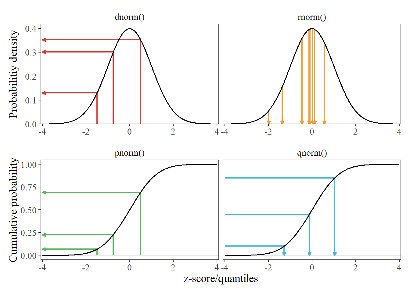
Figure 1: Examples comparing the mappings between different normal distribution functions, given a mean of 0 and standard deviation of 1. Because a standard normal distribution is being used, the terms ‘z-score’ and ‘quantile’ are used interchangeably. Arrows are intended to provide a sense of direction for the examples, in terms of what data are input and output from a given function. dnorm() maps z-scores to their respective density values (point probabilities). rnorm() randomly draws quantiles, weighted by their probability – hence why the most of the 10 random draws are clustered near the peak of the distribution. pnorm() maps a z-score to it’s cumulative probability. qnorm() maps a cumulative probability to a quantile.

And there we have it! A simple visualization to provide a little bit more intuition into R’s distribution functions.