Benchmarking R and Rcpp
A speed comparison.
At the UW Data Science Center we’ve been talking speed lately. Generally R is considered a somewhat slow language (though I’m not sure that’s fair). However, there are some excellent packages and interfaces that can drastically speed up R. For example, the Rcpp package acts as an interface between R and C++, thereby allowing useRs to drastically speed-up analysis – or at least that’s the idea.
In this post I explore the relative speeds of equivalent R and Rcpp functions to see if we really can speed up an arbitrary function by using C++ on the back end.
Libraries
library(tidyverse)## Warning: package 'tidyverse' was built under R version 3.6.2## Warning: package 'tidyr' was built under R version 3.6.2## Warning: package 'dplyr' was built under R version 3.6.2library(Rcpp)
options(tibble.width = Inf)R equations
First, I’m going to make some R equations. We don’t really care what these functions are for the purposes of this exercise. But it one is curious, these equations are very, very loosely based on specific yield relationships, as a function of water table depth and microtopography. The main function being test is: full_balance.
sy <- function(x, cond) {
  out <- ifelse(cond < x, 1, 0)
  out <- 1 - (sum(out) / length(x))
  ifelse(out <= 0.01, 0.01, out)
}

new_cond <- function(curr, addit, subtrac, microt) {
  sy_cond <- sy(microt, curr)
  curr + (addit + subtrac) / sy_cond
}

full_balance <- function(iterations, initial, addition, subtraction, add_sd,
  sub_sd, microtopo) {
  #Initialize
  N <- length(addition) #rows
  M <- iterations #columns
  out <- matrix(nrow = N, ncol = M)
  out[1,] <- initial
  add_error <- matrix(rep(addition, times = M) + rnorm(N * M, 0, add_sd),
    nrow = N, ncol = M, byrow = FALSE)
  sub_error <- matrix(rep(subtraction, times = M) + rnorm(N * M, 0, sub_sd),
    nrow = N, ncol = M, byrow = FALSE)
  #Execute
  for(i in 1:iterations) { #columns
    for(j in 2:length(addition)) { #rows
      out[j, i] <- new_cond(out[j - 1, i], add_error[j, i], sub_error[j, i],
        microtopo)
    }
  }
  #Return
  as.data.frame(out)
}
C++ (Rcpp) equations
Similar functions to those above, but implemented in C++ via the Rcpp package. I should note that I’m not a C++ programmer, so I tried my best to match the functions of the two languages. The main function being test is: full_balance_cpp.
#include <Rcpp.h>
using namespace Rcpp;

// [[Rcpp::export]]
double sy_cpp(NumericVector x, double cond) {
  //Declare
  int N = x.length();
  NumericVector cond_sum(N);
  double out;
  //First ifelse()
  // Short-hand form:
  for(int i = 0; i < N; i++) {
    cond_sum[i] = (cond < x[i] ? 1 : 0);
  }
  //`out` line
  out = 1 - (sum(cond_sum) / N);
  //Second ifelse()
  if(out <= 0.01) {
    out = 0.01;
  }
  //Explicit return statement
  return out;
}

// [[Rcpp::export]]
double new_cond_cpp(double curr, double addit, double subtrac,
  NumericVector microt) {
  //Declare
  double sy_cond;
  double out;
  //Execute
  sy_cond = sy_cpp(microt, curr);
  out = curr + (addit + subtrac) / sy_cond;
  //Return
  return out;
}

// [[Rcpp::export]]
DataFrame full_balance_cpp(int iterations, double initial,
  NumericVector addition, NumericVector subtraction, double add_sd,
  double sub_sd, NumericVector microtopo) {
  //Declare
  int N = addition.length(); //Rows
  int M = iterations; //Columns
  NumericMatrix add_error(N, M);
  NumericMatrix sub_error(N, M);
  NumericMatrix out_mat(N, M);

  //Initialize
  //Set initial conditions for each iteration
  for(int i = 0; i < M; ++i) {
    out_mat(0,i) = initial; //Note `out()` instead of `out[]` for indexing matrices
  }

  //Execute
  //Matrix of observations with error
  for(int i = 0; i < M; ++i) {
    add_error(_, i) = addition + rnorm(N, 0 , add_sd);
    sub_error(_, i) = subtraction + rnorm(N, 0 , add_sd);
  }
  //Loop through each set of observations
  for(int i = 0; i < M; ++i) {
    for(int j = 1; j < N; ++j){
      out_mat(j, i) = new_cond_cpp(out_mat(j - 1, i), add_error(j, i),
        sub_error(j, i), microtopo);
    }
  }

  //Return a dataframe of results
  //Explicit coercion to a different, compatable type following the pattern:
  // as<type>(object)
  DataFrame out = as<DataFrame>(out_mat);
  return out;
}
Data
Now let’s generate some data to use with our functions. Again, we don’t really care what the data actually means – it’s just an example.
per_obs <- 1:200
per_n <- length(per_obs)

add_means <- 0.5 * (sin(seq(0, 2 * per_n / 100 * pi, length.out = per_n))) +
  abs(rnorm(per_obs))
add_means <- ifelse(add_means < 0 , 0, add_means)
sub_means <- 0.75 * (cos(seq(0, 2 * per_n / 100 * pi, length.out = per_n)) - 2) +
  abs(rnorm(per_obs))
sub_means <- ifelse(sub_means > 0 , 0, sub_means)

add_sds <- 1
sub_sds <- 1

init_cond <- 0

micro <- map2(.x = c(-4, -2, 0, 2, 5), .y = c(3, 1, 2, 4, 1),
  ~ rnorm(2000, .x, .y)) %>%
  simplify()
But what does the data look like (just for fun)?
qplot(per_obs, add_means + sub_means) + theme_bw()
qplot(micro, geom = "density") + theme_bw()
Benchmarking
Here I’m using the bench package to iterate over different parameter sets, so we may get an idea of how the two equivalent functions respond to changes in function conditions. Pretty cool package.
Run the benchmarks
micro_maker <- function(obs) {
  map2(.x = c(-4, -2, 0, 2, 5), .y = c(3, 1, 2, 4, 1),
  ~ rnorm(obs, .x, .y)) %>%
  simplify()
}

iter_maker <- function(iters) {
  iters
}

bench_press <- bench::press(
  obs = c(10, 100, 1000),
  iters = c(1, 10, 100, 1000),
  {
    iterations = iter_maker(iters)
    microtopo = micro_maker(obs)
    bench::mark(
      R = full_balance(iterations, init_cond, add_means, sub_means, add_sds,
        sub_sds, microtopo),
      Rcpp = full_balance_cpp(iterations, init_cond, add_means, sub_means,
        add_sds, sub_sds, microtopo),
      check = FALSE,
      max_iterations = 20
    )
  }
)
Investigate the results of the benchmark
Now that we have the results, let’s take a quick look at the output.
bench_press %>%
  mutate(expression = attr(expression, "description")) %>%
  select(-`gc/sec`, -n_itr, -n_gc, -total_time) %>%
  print(n = nrow(.))
## # A tibble: 24 x 7
## expression obs iters min median `itr/sec` mem_alloc
## <chr> <dbl> <dbl> <dbl> <dbl> <dbl> <dbl>
## 1 R 10 1 0.00190 0.00258 321. 770160
## 2 Rcpp 10 1 0.000187 0.000341 2311. 104088
## 3 R 100 1 0.00318 0.00377 234. 4627848
## 4 Rcpp 100 1 0.000361 0.000445 2112. 820488
## 5 R 1000 1 0.0236 0.0247 38.0 45122144
## 6 Rcpp 1000 1 0.00287 0.00319 208. 7984488
## 7 R 10 10 0.0173 0.0206 46.7 5913768
## 8 Rcpp 10 10 0.000719 0.000818 1092. 1016184
## 9 R 100 10 0.0410 0.0477 19.7 46701968
## 10 Rcpp 100 10 0.00335 0.00383 186. 8180184
## 11 R 1000 10 0.281 0.314 3.19 454901000
## 12 Rcpp 1000 10 0.0388 0.0446 22.5 79820184
## 13 R 10 100 0.197 0.200 4.78 58746024
## 14 Rcpp 10 100 0.00707 0.00755 89.3 10139688
## 15 R 100 100 0.611 0.611 1.64 462609712
## 16 Rcpp 100 100 0.0562 0.0687 14.4 81779688
## 17 R 1000 100 2.24 2.24 0.447 4594637656
## 18 Rcpp 1000 100 0.426 0.457 2.19 798179688
## 19 R 10 1000 2.23 2.23 0.448 588214760
## 20 Rcpp 10 1000 0.0655 0.0764 9.86 101370888
## 21 R 100 1000 4.29 4.29 0.233 4627849424
## 22 Rcpp 100 1000 0.387 0.394 2.54 817770888
## 23 R 1000 1000 23.3 23.3 0.0428 45325385200
## 24 Rcpp 1000 1000 3.77 3.77 0.265 7981770888Interesting. Looks like Rcpp is, indeed, faster. Also interesting is the mem_alloc column. It seems that Rcpp uses much less memory.
Visualize the results of the benchmark
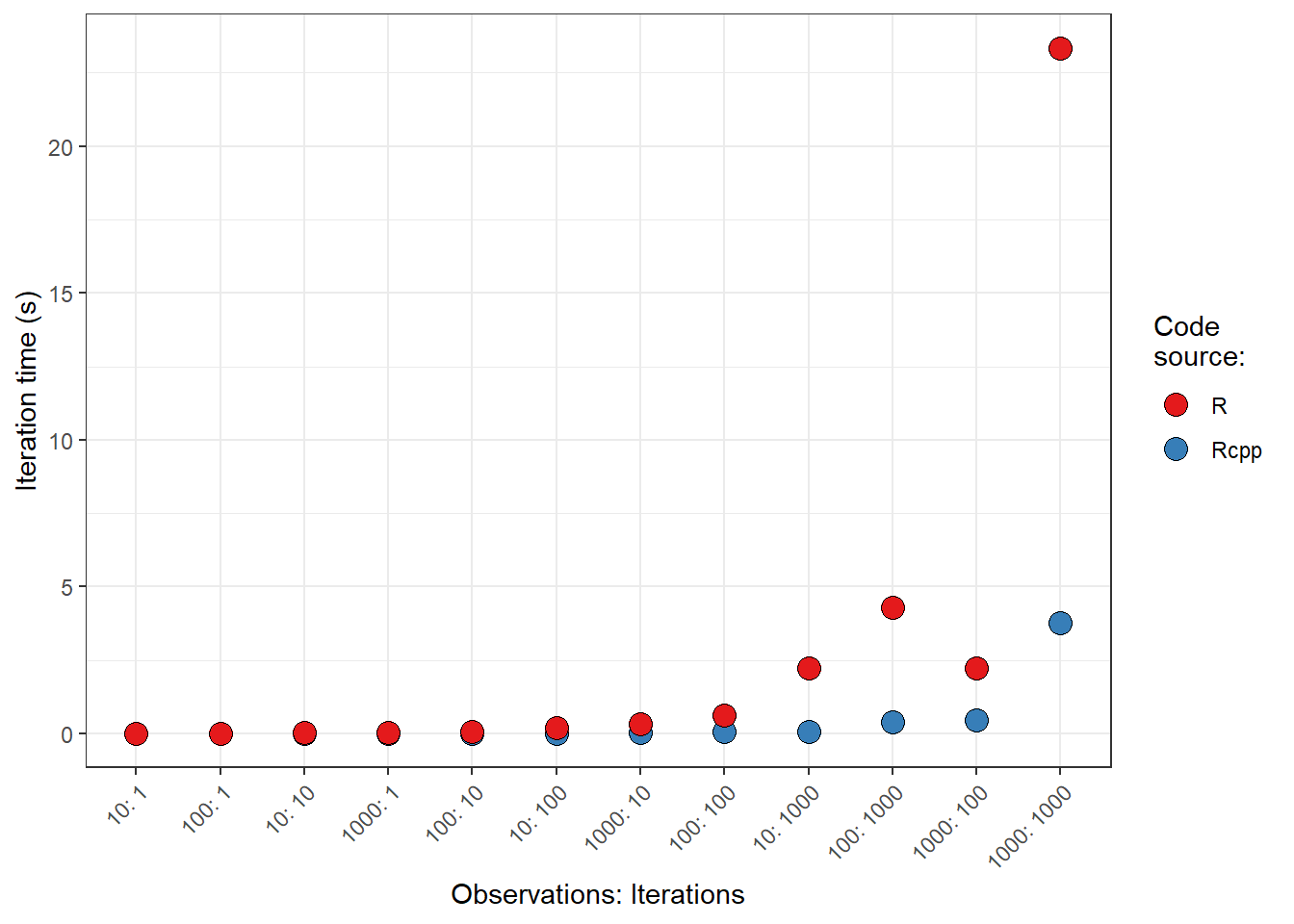
Finally, let’s take a look at a visual representation, comparing the two code sources across the different parameter sets. Points indicate the median iteration time. Note: variance in run times are so small that they cannot be seen at the scales provided.
bp_time_df <- bench_press %>%
  mutate(rows = 1:n(),
    expression = attr(expression, "description"))

bp_time_df %>%
  group_by(obs, iters, expression) %>%
  summarise(median = first(median)) %>%
  ungroup() %>%
  mutate(combo = paste0(obs, ": ", iters)) %>%
  arrange(median, combo) %>%
  mutate(combo = fct_inorder(combo)) %>%
  ggplot(aes(combo, median, fill = expression)) +
  geom_point(shape = 21, size = 4) +
  labs(x = "Observations: Iterations",
    y = "Iteration time (s)",
    fill = "Code\nsource:") +
  theme_bw() +
  theme(axis.text.x = element_text(angle = 45, hjust = 1)) +
  scale_fill_brewer(palette = "Set1")
It looks like there is a big spike in the differences between the two code sources as the number of “iterations” increases (not that I defined that term super well for you all, but as a relative metric, hopefully the gains in speed are at least relatively appreciated between R and Rcpp).